# remotes::install_github('r-spatial/sf')
library(sf)

# remotes::install_github('r-lidar/lidR')
library(lidR)

# remotes::install_github('rspatial/terra')
library(terra)

# remotes::install_github('tylermorganwall/rayshader')
library(rayshader)Varina LandLab LIDAR
The Varina LandLab is a parcel of land in Henrico County, VA acquired by the Capital Region Land Conservancy in 2021. Several Civil War battles were fought in the vicinity (which could mean cool features like earthworks!), but what we’re interested in with this exercise is figuring out a more-precise location of a small creek-side cabin demolished in 1982.
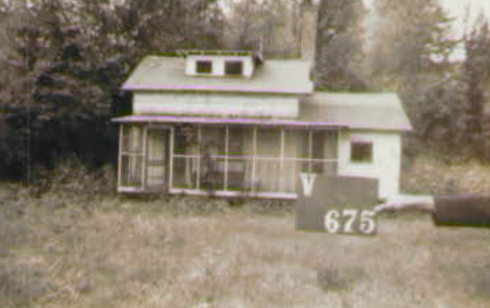
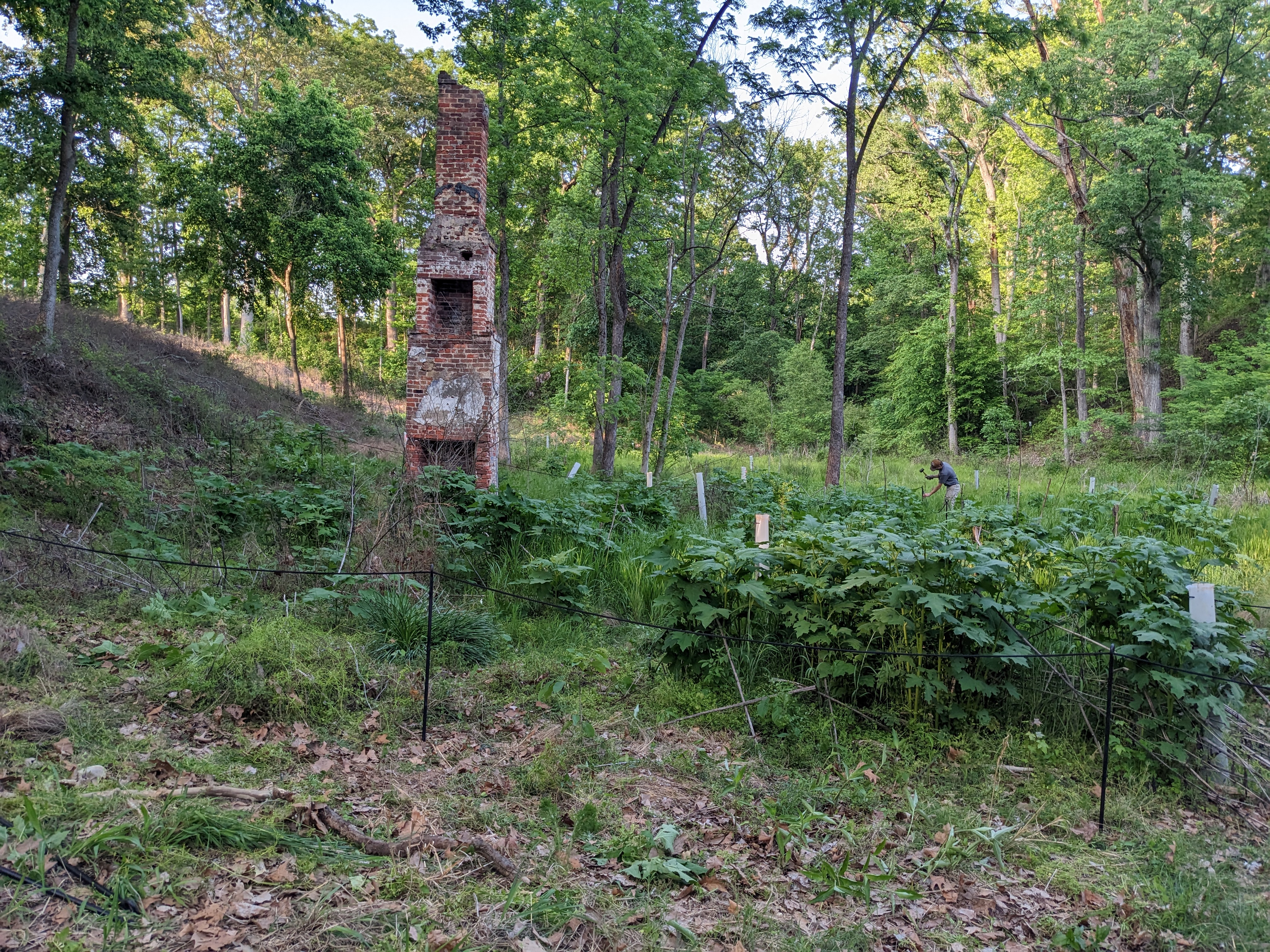
All that currently remains is the chimney; the photo below would have been taken to the left of the photo above.
Working with LIDAR
The United States Geological Survey (USGS) provides LIDAR point cloud data from throughout the United States. You can click around and see what’s available using their LidarExplorer tool.
Point cloud data are provided in blocks, or tiles. What interests us are those tiles surrounding the LandLab. At the time of this writing, the most-recent LIDAR surveys were conducted in December 2019 – this is before the parcel was acquired by CLRC (2021) and most of the work around the parcel, including prescribed burns (2022), was conducted. The associated tiles are linked here:
- https://www.sciencebase.gov/catalog/item/5fe758aad34ea5387debaa59
- https://www.sciencebase.gov/catalog/item/5fe758aad34ea5387debaa57
- https://www.sciencebase.gov/catalog/item/5fe7589bd34ea5387debaa1b
- https://www.sciencebase.gov/catalog/item/5fe7589bd34ea5387debaa19
If you’d like to follow along with the analysis, download and put them all in the same folder (we’ll call it local_folder in the code). The R package we’ll be using (lidR) has really good group operations using a “LAScatalog”; putting the files in the same directory allows us to treat them this way.
My programming and analysis background is in R, so I’m just going to plow ahead and, as noted above, use the lidR package. lidR is excellently documented via their GitHub pages book; most of my code below is a slight adaptation of the workflows that they published.
I’ll also use the sf package to extract information about the coordinate reference system (CRS) and projection of the LIDAR data, the terra package to create a terrain model, and the rayshader package to throw some light across the terrain model. This “raytracing” really helps pick up subtle features.
I’ll be running this on R 4.3, but, as I use the base pipe operator “|>”, it should work with any version greater than 4.1. All of the packages can be installed using install.packages, but it may be useful to install them via the remotes package to be up-to-date with the most recent additions.
Getting a point of reference
First, we’re going to grab the LIDAR header to get the CRS. We’ll need to convert the latitude/longitude of the cabin to the same CRS and it’ll be easier to transform them than a big .laz file.
las_crs <- st_crs(
  readLASheader(
    file.path(local_folder,
              'deep_bottom_laz',
              'USGS_LPC_VA_SouthamptonHenricoWMBG_2019_B19_18STG955415.laz')
  )
)

las_crs
Coordinate Reference System:
User input: COMPD_CS["NAD83(2011) / UTM zone 18N + NAVD88 height - Geoid12B (metre)",PROJCS["NAD83(2011) / UTM zone 18N",GEOGCS["NAD83(2011)",DATUM["NAD83 (National Spatial Reference System 2011)",SPHEROID["GRS 1980",6378137,298.257222101,AUTHORITY["EPSG","7019"]],AUTHORITY["EPSG","1116"]],PRIMEM["Greenwich",0,AUTHORITY["EPSG","8901"]],UNIT["degree",0.0174532925199433,AUTHORITY["EPSG","9122"]],AUTHORITY["EPSG","6318"]],PROJECTION["Transverse_Mercator"],PARAMETER["latitude_of_origin",0],PARAMETER["central_meridian",-75],PARAMETER["scale_factor",0.9996],PARAMETER["false_easting",500000],PARAMETER["false_northing",0],UNIT["metre",1,AUTHORITY["EPSG","9001"]],AXIS["X",EAST],AXIS["Y",NORTH],AUTHORITY["EPSG","6347"]],VERT_CS["NAVD88 height - Geoid12B (metre)",VERT_DATUM["North American Vertical Datum 1988",2005,AUTHORITY["EPSG","5103"]],UNIT["metre",1,AUTHORITY["EPSG","9001"]],AXIS["Up",UP],AUTHORITY["EPSG","5703"]]]
wkt:
COMPOUNDCRS["NAD83(2011) / UTM zone 18N + NAVD88 height - Geoid12B (metre)",
PROJCRS["NAD83(2011) / UTM zone 18N",
BASEGEOGCRS["NAD83(2011)",
DATUM["NAD83 (National Spatial Reference System 2011)",
ELLIPSOID["GRS 1980",6378137,298.257222101,
LENGTHUNIT["metre",1]]],
PRIMEM["Greenwich",0,
ANGLEUNIT["degree",0.0174532925199433]],
ID["EPSG",6318]],
CONVERSION["UTM zone 18N",
METHOD["Transverse Mercator",
ID["EPSG",9807]],
PARAMETER["Latitude of natural origin",0,
ANGLEUNIT["degree",0.0174532925199433],
ID["EPSG",8801]],
PARAMETER["Longitude of natural origin",-75,
ANGLEUNIT["degree",0.0174532925199433],
ID["EPSG",8802]],
PARAMETER["Scale factor at natural origin",0.9996,
SCALEUNIT["unity",1],
ID["EPSG",8805]],
PARAMETER["False easting",500000,
LENGTHUNIT["metre",1],
ID["EPSG",8806]],
PARAMETER["False northing",0,
LENGTHUNIT["metre",1],
ID["EPSG",8807]]],
CS[Cartesian,2],
AXIS["x",east,
ORDER[1],
LENGTHUNIT["metre",1]],
AXIS["y",north,
ORDER[2],
LENGTHUNIT["metre",1]],
ID["EPSG",6347]],
VERTCRS["NAVD88 height",
VDATUM["North American Vertical Datum 1988"],
CS[vertical,1],
AXIS["up",up,
LENGTHUNIT["metre",1]],
GEOIDMODEL["GEOID12B"],
ID["EPSG",5703]]]There is a lot going on there! The biggest things to note here are that:
- The CRS is NOT WGS 84, “World Geodetic System 1984”, a model of the shape of the Earth that a GPS uses and what we’re thinking in when we say “lat/long”.
- The units of this coordinate system are meters
I didn’t mark the location of the cabin when I was there, but the metadata of the picture above recorded by my phone says that it was taken at 37.40624 degrees north and -77.31064 degrees east. By saying this, we’re thinking in WGS 84; one GIS shorthand for this is the EPSG code 4326. We’ll now tell R that these coordinates represent a point in WGS 84, then convert that point to the CRS of the LIDAR data.
photo_point <-
  # "These X-Y coordinates..."
  c(-77.31064, 37.40624) |>
  # "...are a point..."
  st_point() |>
  # "...in WGS 84..."
  st_sfc(crs = 4326) |>
  # "...that should be transformed to the LIDAR CRS."
  st_transform(las_crs)

photo_point
Geometry set for 1 feature
Geometry type: POINT
Dimension: XY
Bounding box: xmin: 295492.6 ymin: 4142445 xmax: 295492.6 ymax: 4142445
Projected CRS: NAD83(2011) / UTM zone 18N + NAVD88 height - Geoid12B (metre)POINT (295492.6 4142445)Ta-da! Our point is now something like 4100 km north of the equator and 205 km west of the -75 degree longitudinal meridian (295492 - 500000) on a North-America-centric model of the planet Earth. Don’t think about it too hard, unless you really, really want to.
Let’s now read in our LAScatalog, but, in order to save memory, select only a small portion (a circle with a 30 meter radius around where I took the picture).
db_lidar <- readLAScatalog(
  file.path(
    local_folder,
    'deep_bottom_laz'
  )
) |>
  clip_circle(xcenter = 295492.6, ycenter = 4142445, radius = 30)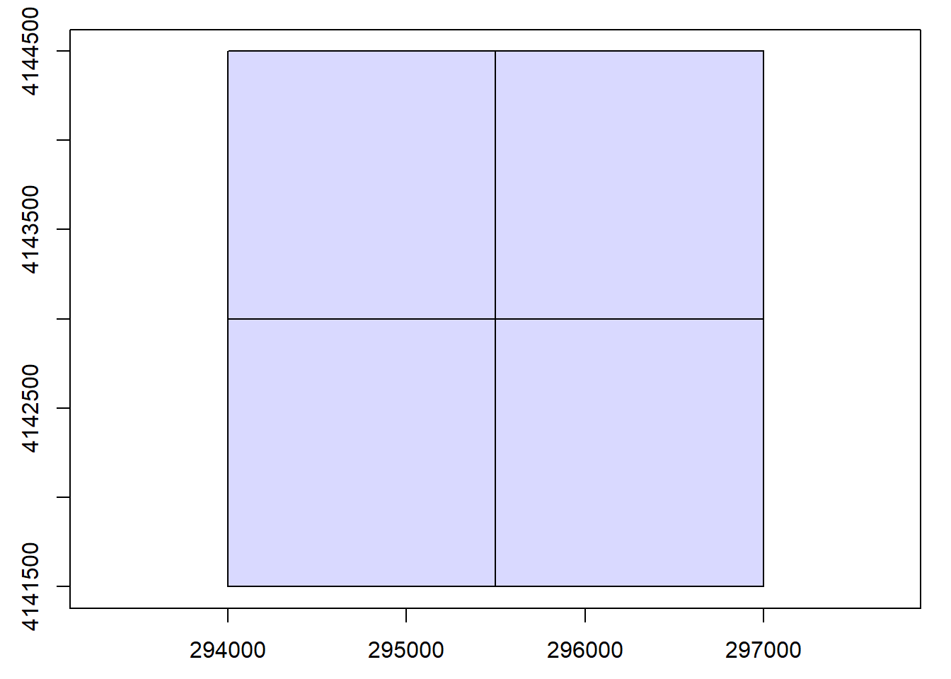
Chunk 1 of 1 (100%): state ✓Seeing what we’re working with
What does that look like? COLORFUL TREES (AND GROUND!)!
plot(db_lidar)This is the neat part about LIDAR data – we can get an idea about what the tree canopy looks like using the “first returns”, those points of light that hit something high and bounced back to the airplane first…
filter_first(db_lidar) |>
  plot()
…or what the ground looks like by using “last returns”, the light that went the farthest.
filter_ground(db_lidar) |>
  plot()
“…enhance.”
We really want to drill down on what the ground looks like. To do this, we’ll “rasterize” the LIDAR points. This basically means that we’ll create a grid with some resolution (I’m going to use 1/2 meter), fill in the points for which we have values and then interpolate the rest. I’m more-or-less following the lidR book from this point on.
dtm_tin <- rasterize_terrain(db_lidar, res = 0.5, algorithm = tin())

plot(dtm_tin)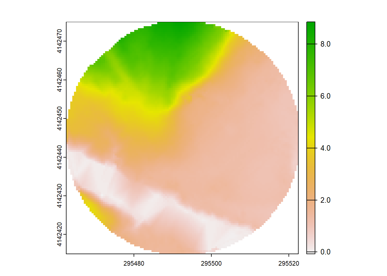
Now, we’ll create the digital terrain model.
dtm_prod <- terrain(dtm_tin, v = c("slope", "aspect"), unit = "radians")

dtm_hillshade <- shade(slope = dtm_prod$slope, aspect = dtm_prod$aspect)

plot(dtm_hillshade, col = gray(0:50/50), legend = FALSE)
plot(photo_point, add = T, col = 'red')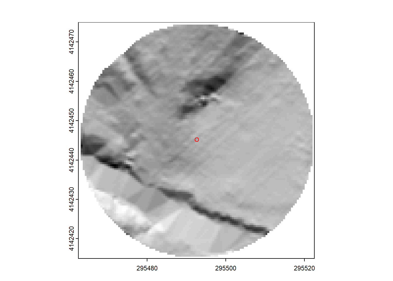
There are some artifacts in there, but look at the hill above the red circle (where I took the picture). Now, if you look closely, you can see that it is flat between the picture and the hill! That’s the foundation – or at least remnants thereof – of our cabin!
Just ball-parking here, but this us my (very coarse) outline.
foundation <- rbind(
  c(-77.31063, 37.40627),
  c(-77.31066, 37.40629),
  c(-77.31060, 37.40632),
  c(-77.31057, 37.40630),
  c(-77.31063, 37.40627)
) |>
  list() |>
  st_polygon() |>
  st_sfc(crs = 4326) |>
  st_transform(las_crs)

plot(dtm_hillshade, col = gray(0:50/50), legend = FALSE)
plot(photo_point, add = T, col = 'red')
plot(foundation, add = T)
Make it POP
I’m going to do some raytracing (move the “sun” around) to exaggerate features.
dtm <- raster::raster(dtm_tin)
elmat <- raster_to_matrix(dtm)

map <- elmat |>
  # make the sun come from the east (90 deg) and ramp up the colors
  sphere_shade(sunangle = 90, texture = 'unicorn', colorintensity = 10) |>
  add_shadow(ray_shade(elmat))

plot_map(map)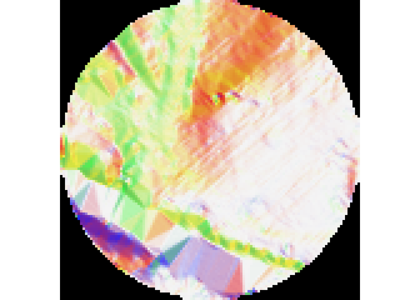
plot_3d(map, elmat, zscale = 0.4)Conclusion
So, there we have it: A general idea of where the cabin, thought to possibly be a ferry keeper’s house, might have stood over forty years ago. Definitely not exact, but it’s interesting to see that we can pick up the remnants of something that hasn’t existed for nearly half of a century by using something so sci-fi as to asking an airplane to bounce beams of light off of the ground.
This just means that I’ll have to take ask one of the CLRC staff to head out there with a GPS in hand, actually mark the chimney, and see how accurate my estimate might be. I’d do it myself, but the site has been (smartly) roped off in hopes of further preservation.
After all, conservation, contextualization, and visualization of history is what we’re after.